Perceptron

v. 1.5 March 2015

Home

Perceptron upholds the infinite, circular flow of pixels (their colors), or in other words, visual images. The visual images evolve quickly, slowly or endlessly depending from the geometric transformations that are occurring between the two stages along the flow, the screen and the buffer memory.

Perceptron uses 4 matrices of equivalent format: screen, buffer (temporary screen contents holder), lookup table, and gradient matrix. All 4 matrices are used in coordination, that is, we focus on a single element from each of the 4 matrices at a given time in order to update a single pixel of the buffer. For speed purposes, all matrices are stored in the form of one-dimensional arrays.

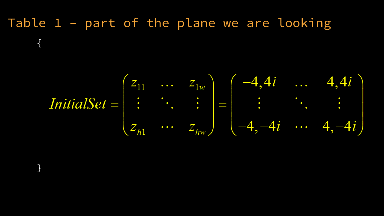
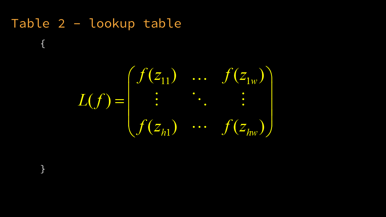
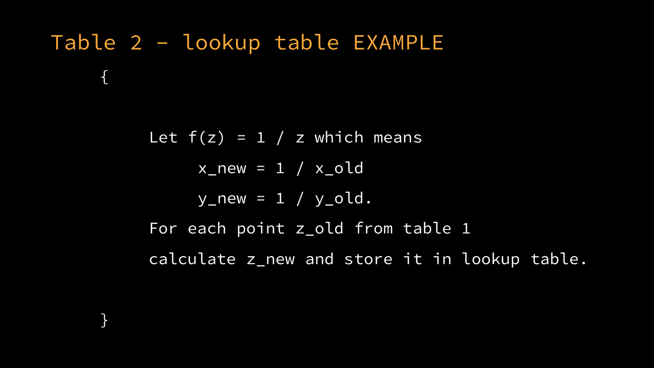
The flow of visual images starts with the screen matrix and follows to the buffer matrix. The screen represents the portion of the complex plane around the coordinate zero, no bigger than the circle of radius r = 3. The first or initial visual image (frame 0) needs to be copied (“mapped”) from the screen to the buffer. The buffer will fill its element (pixel) at the position z = (x, y) by reading the position z’ = f(z) at the screen. The complex number z’ is precalculated and stored in the lookup table at the position z.

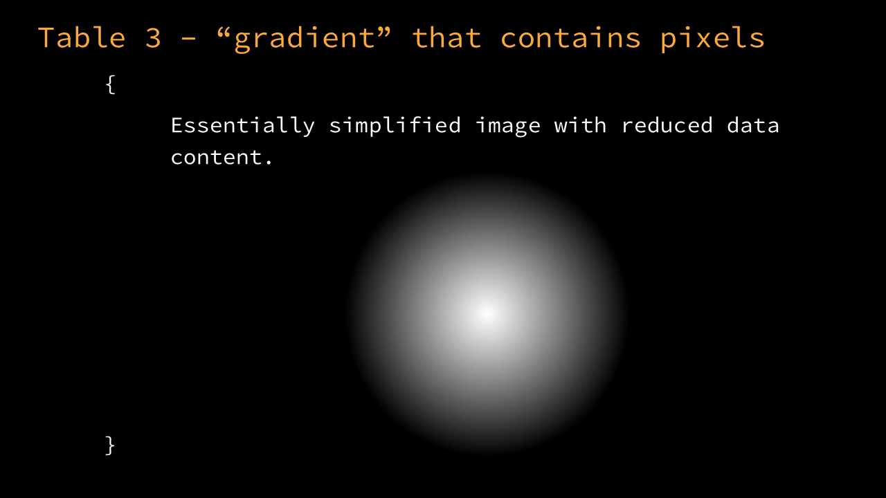
Next, we test to see whether the point z’ is inside the limit circle of radius r = 1 or outside (depending from the boundary condition). If it is within the circle, the color read at the screen position z’ is color inverted and copied to the buffer at position z. If the point z’ is outside of the limit circle, some color is added to the existing pixel color found at the screen location z’, after which it is color inverted, and written to the buffer at position z. The added color depends from various coloring functions. Primarily, it is a color value (“shadow intensity”) taken from the gradient matrix at the position z. The gradient matrix is precalculated and filled with a shape such as the radial (round) shadow, black in the middle and gradually whiter towards the edge. When all pixels of the buffer are filled, the buffer is copied to the screen directly. Over several cycles, this creates a gray-scale Julia fractal with black and white contours.  

The mentioned color inversion affects pixels read at the screen position z’ both when z’ is inside the limit circle and when z’ is outside the limit circle (that is, regardless of the boundary condition check). We call it the total color inversion that affects the entire flow of visual images (all screen contents). You can find the option to disable the total inversion in the help menu. The partial color inversion refers to the situation when the total color inversion is enabled, but you want to color invert the fractal that you have in front of you on the screen. The total color inversion is responsible for the concentric, interchanging Julia contours (e.g. black and white) and for the flicker of the Julia lake. The partial color inversion is a switch that replaces the black contours with white and white with black.

Let us step back to the situation right after the boundary condition check. If the point z’ is beyond the screen matrix size, the “reflection transform” moves it inside (contracts it) by the application of somewhat nonsensical linear functions. The color is obtained from the screen after all, color inverted, and passed on to the buffer. This creates multiple “reflections”, simple copies of Julia fractal portions (fragments) that form IFS fractals. The linear functions are equivalent to the affine transformations used to create IFS fractals in the ordinary fractal generators.

A single cycle is complete when the buffer sends (copies) its contents to the screen as they are. This initiates a new cycle of geometric transformations from the screen to the buffer. Over the course of many cycles, the exquisite combination of Julia and IFS fractals emerges. The age of a video feedback fractal is expressed by the number of cycles performed, which is also known as the number of iterations. The age determines the recursive depth (e.g. number of concentric Julia contours added inwardly).

The combined Julia and IFS fractals sometimes occur as the effect of branch cuts of certain complex functions when they are used in the conventional fractal generators (such as Fractint and UltraFractal). See the fantastic artwork by Dan Wills at https://ultraiterator.blogspot.com.